Mean Reversion

Mean Reversion in Time Series: What it is and Trading Strategies
Time series data is simply a collection of observations generated over time. For example, the speed of a race car at each second, daily temperature, weekly sales figures, stock returns per minute, etc.
In the financial markets, a time series tracks the movement of specific data points, such as a security’s price over a specified period of time, with data points recorded at regular intervals. A time series can be generated for any variable that is changing over time.
Further, mean reversion is a simple concept of the stock prices eventually reverting to the mean after deviating from the mean for a certain period of time due to any significant changes in the economy, the organization etc.
Let us find out more about mean reversion in time series with this blog that covers:
What is time series analysis?
A time series is a sequence of observations indexed over time. In trading, time series forms an important part as it is used to track down the prices of a security over a period of time.
For instance, movement of a security’s price, over a specific period of time recorded at a regular interval.
Components of a time series
1. Trend: Trend may show growth or decline in a time series over a long period.
2. Cycles: These are long term oscillations occurring in a time series. These movements generally extend from five to twelve years or more.
3. Seasonality: The periodic fluctuation of time series within a certain period. These fluctuations form a pattern that tends to repeat from one seasonal period to another. Unlike cycles, seasonal behaviour is very strictly regular, meaning there is a precise amount of time between the peaks and troughs of the data.
4. Irregular Fluctuation: These are sudden changes occurring in a time series which are unlikely to repeat. These cannot be explained by trend, seasonal or cyclic movement. This component is sometimes called as random movements in a time series.
Now, time series analysis implies analyzing a time series data to understand its characteristics, design and framework in order to draw inferences from it. Time series analysis has many applications which include yield projections, inventory studies, economic forecasting, sales forecasting etc.
Different methods through which time series analysis can be done include simple forecasting and smoothing models, correlation analysis methods, and ARIMA model.
Let us now take a look at the graph below, which represents the daily closing price of Aluminium futures over a period of 93 trading days, which is a Time Series.
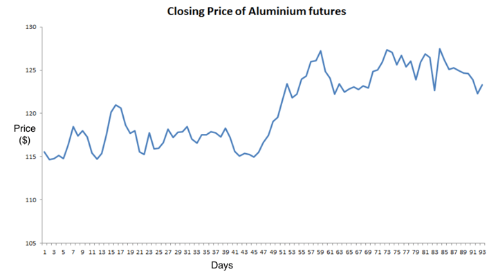
Close price
Time series analysis is important because it facilitates in:
Identifying the nature of the phenomenon represented by the sequence of observations in the data.
Forecasting future values of the time series variable.
Comparing different time series.
What is mean reversion?
Mean reversion theory suggests that considerable deviations in security prices tend to return to their historical mean.
In other words, if the price moves too far away from its long term average, it will revert to its average. This theory considers only the extreme changes and does not include the normal growth and other market events that take place.
When the current market price is less than the average price, traders purchase the stock with an expectation that the price will rise. Similarly, When the price is above the average price, investors will sell that security expecting the price to pull back to mean. Pairs trading strategy is based on the mean reversion theory.
For an example, let us assume that the 1 year average price of Stock ABC is $125 and the stock is trading at $150. There may be a gradual increase in the price of the stock over the year due to strong fundamentals but if the stock price increases by 8% within a trading day to $162, then one might short the stock assuming it will return to its long term mean and book a profit.
Why does mean reversion trading work?
Mean reversion trading strategy works since the price is always moving or oscillating around the mean. The reason for the prices reverting to the mean is mainly the sentiments of the traders when the prices deviate from the norm.
Whenever the stock’s price rises in a trend, the traders and investors buy the stocks immediately to avoid missing out on opportunities that a risen price can give. Hence, the demand is more than the supply. This increase in demand also moves the price up further.
As the price continues to rise, more and more traders come into the picture to buy the stock until it reaches a peak where the traders finally start to sell. Now, the role reversal takes place and the supply becomes more than the demand.
In such a situation, the price begins to fall. Forseeing a fall in the price, the majority of the traders start to sell their stocks in fear of losing which leads to surplus in the supply of stocks and the price declines even faster.
Now, at a very low price, some traders begin to buy the stock again pushing the price slightly up. This leads to a balance and hence, the price reverts to the mean.
How does a stock undergo mean reversion in time series?
In the case of mean reversion in time series, the stationarity test plays an integral role.
The stationary test will help you analyse if the time series is stationary or is non-stationary. The time series will be stationary if its mean and variance are constant over time.
Furthermore, a stationary time series will be mean reverting in nature, i.e., it will not drift too far away from its mean because of its finite constant variance.
Whereas, a non-stationary time series, on the contrary, will have a time varying variance or a time varying mean or both, and will not tend to revert back to its mean.
Relevance of stationarity
In the financial industry, traders take advantage of the stationary time series by placing orders when the price of security deviates considerably from its historical mean, speculating the price to revert to its mean.
Shown below is a plot of an asset which is a non-stationary time series with a deterministic trend (Yt = α + βt + εt) represented by the blue curve and its detrended stationary time series (Yt - βt = α + εt) represented by the red curve.